Social Media Mining With R Download
A Guide to Mining and Analysing Tweets with R
Simple Steps to Writing an Insightful Twitter Analytics Report
![]()

Twitter provides us with vast amounts of user-generated language data — a dream for anyone wanting to conduct textual analysis. More than that, tweets allow us to gain insights into the online public behaviour. As such, analysing Twitter has become a crucial source of information for brands and agencies.
Several factors have given Twitter considerable adv a ntages over other social media platforms for analysis. First, the limited character size of tweets provides us with a relatively homogeneous corpora. Second, the millions of tweets published everyday allows access to large data samples. Third, the tweets are publicly available and easily accessible as well as retrievable via APIs.
Nonetheless, extracting these insights still requires a bit of coding and programming knowledge. This is why, most often, brands and agencies rely on easy-to-use analytics tools such as SproutSocial and Talkwalker who provide these insights at a cost in just one click.
In this article, I help you to break down these barriers and provide you with a simple guide on how to extract and analyse tweets with the programming software R.
Here are 3 reasons why you might chose to do so:
- Using R is for free, i.e. you will be able to produce a Twitter Analytics Report for free and learn how to code at the same time!
- R allows you infinite opportunities for analysis. Using it to analyse Twitter therefore allows you to conduct tailor-made analysis depending on what you wish to analyse instead of relying on a one-size-fits-all report
- R allows you to analyse any Twitter account you want even if you don't have the log-in details. This is a huge advantage compared to many analytics tools that require you to have the log-in details in order to analyse the information in the first place.
Convinced? Let's get started, then!
STEP 1: Getting your Twitter API access
In order to get started, you first need to get a Twitter API. This will allow you to retrieve the tweets — without it, you cannot do anything. Getting a Twitter API is easy. First make sure you have a Twitter account, otherwise create one. Then, apply for a developer account via the following website: https://developer.twitter.com/en/apply-for-access.html. You'll need to fill in an application form, which includes explaining a little a bit more what you wish you analyse.
Once you application has been accepted by Twitter (which doesn't take too long), you'll receive the following credentials that you need to keep safe:
- Consumer key
- Consumer Secret
- Access Token
- Access Secret
STEP 2: Mining Tweets
Once you have the information above, start R and download the package "rtweet", which I will use to extract the tweets.
          install.packages("rtweet")
library (rtweet)
Then, set up the authentification to connect to Twitter. You do this by entering the name of your app, consumer key and consumer secret — all of it is information you have received when applying for the Twitter API. You will be re-directed to a Twitter page and asked to accept the authentification. Once this is done, you can return to R and start the analysis of your tweets!
          twitter_token <- create_token(
            app = ****,
            consumer_key = ****,
            consumer_secret = ****,
            set_renv = TRUE)
Searching for tweets
Depending on the analysis you wish to perform, you may want to search for tweets that contain a specific word or hashtag. Note that you can only extract tweets from the past 6 to 9 days, so keep this in mind for your analysis.
To do this, simply use the search_tweets function followed by a few specifications: the number of tweets to extract (n), whether or not to include retweets and the language of the tweets. As an example, see the line of code below.
climate <- search_tweets("climate", n=1000, include_rts=FALSE, lang="en") Search for a specific user account
Alternatively, you may want to analyse a specific user account. In this case, use the get_timeline function followed by the twitter handle and number of tweets you wish to extract. Note that here you can only extract the last 3200 tweets.
In this example, I chose to exract the tweets of Bill Gates. The advantage here is that Bill Gates' account counts 3169 tweets overall, which is under the 3200 threshold.
Gates <- get_timeline("@BillGates", n= 3200) STEP 3: Analyse the tweets
In this part, I show you 8 key insights you should include in every Twitter Analytics Report. To do this, let's delve into the Twitter account of Bill Gates a bit more!
1. SHOW WHAT WORKS BEST AND WHAT DOESN'T
The first part of any report should deliver clear information as to what worked best and what didn't. Finding out the best and least performing tweets gives a quick and clear overall picture of the account.
In order to do this, you first need to distinguish between organic tweets, retweets and replies. The following line of code shows you how to remove the retweets and replies from your sample to keep only the organic tweets — content-wise, these are the ones you want to analyse!
          # Remove retweets
Gates_tweets_organic <- Gates_tweets[Gates_tweets$is_retweet==FALSE, ]                    # Remove replies
Gates_tweets_organic <- subset(Gates_tweets_organic, is.na(Gates_tweets_organic$reply_to_status_id))
Then, you'll want to analyse engagement by looking at the variables: favorite_count (i.e. the number of likes) or retweet_count (i.e. the number of retweets). Simply arrange them in descending order (with a minus "-" before the variable) to find the one with the highest number of likes or retweets or ascending order (without the minus) to find the one with lowest number of engagements.
          Gates_tweets_organic <- Gates_tweets_organic %>% arrange(-favorite_count)
Gates_tweets_organic[1,5]          Gates_tweets_organic <- Gates_tweets_organic %>% arrange(-retweet_count)
Gates_tweets_organic[1,5]
2. SHOW THE RATIO OF REPLIES/RETWEETS/ORGANIC TWEETS
Analysing the ratio of replies, retweets and organic tweets can tell you a great deal about the type of account you're analysing. No one likes a Twitter account that exclusively retweets for instance, without any individual content. Finding a good ratio of replies, retweets and organic tweets is therefore a key metric to monitor if one wishes to improve the performance of his or her account.
As a first step, make sure to create three different data sets. As you've already created a dataset containing only the organic tweets in the previous steps, simply now create a dataset containing only the retweets and one containing only the replies.
          # Keeping only the retweets
Gates_retweets <- Gates_tweets[Gates_tweets$is_retweet==TRUE,]          # Keeping only the replies
Gates_replies <- subset(Gates_tweets, !is.na(Gates_tweets$reply_to_status_id))
Then, create a separate data frame containing the number of organic tweets, retweets, and replies. These numbers are easy to find: they are the number of observations for your three respective datasets.
          # Creating a data frame
data <- data.frame(
            category=c("Organic", "Retweets", "Replies"),
            count=c(2856, 192, 120)
)
Once you've done that, you can start preparing your data frame for a donut chart as shown below. This includes adding columns that calculate the ratios and percentages and some visualisation tweaks such as specifying the legend and rounding up your data.
          # Adding columns
data$fraction = data$count / sum(data$count)
data$percentage = data$count / sum(data$count) * 100
data$ymax = cumsum(data$fraction)
data$ymin = c(0, head(data$ymax, n=-1))          # Rounding the data to two decimal points
data <- round_df(data, 2)          # Specify what the legend should say
Type_of_Tweet <- paste(data$category, data$percentage, "%")          ggplot(data, aes(ymax=ymax, ymin=ymin, xmax=4, xmin=3, fill=Type_of_Tweet)) +
            geom_rect() +
            coord_polar(theta="y") +
            xlim(c(2, 4)) +
            theme_void() +
            theme(legend.position = "right")

3. SHOW WHEN THE TWEETS ARE PUBLISHED
Thanks to the date and hour extracted with each tweet, understanding when Bill Gates tweets most is very easy to analyse. This can give us an overall overview of the activity of the account and can be a useful metric to be analysed against the most and least performing tweets.
In this example, I analyse the frequency of tweets by year. Note that you can also do so by month by simply changing "year" to "month" in the following line of code. Alternatively, you can also analyse the publishing behaviour by hour with the R packages hms and scales.
          colnames(Gates_tweets)[colnames(Gates_tweets)=="screen_name"] <- "Twitter_Account"          ts_plot(dplyr::group_by(Gates_tweets, Twitter_Account), "year") +
            ggplot2::theme_minimal() +
            ggplot2::theme(plot.title = ggplot2::element_text(face = "bold")) +
            ggplot2::labs(
            x = NULL, y = NULL,
            title = "Frequency of Tweets from Bill Gates",
            subtitle = "Tweet counts aggregated by year",
            caption = "\nSource: Data collected from Twitter's REST API via rtweet"
            )

4. SHOW FROM WHERE THE TWEETS ARE PUBLISHED
Analysing the source of the platform from which tweets are published is another cool insight to have. One of the reasons is that we can to a certain extent deduct whether or not Bill Gates is the one tweeting or not. As a result, this helps us define the personality of the tweets.
In this step, you're interested in the source variable collected by the rtweet package. The following line of codes shows you how to aggregate this data by type of source and count the frequency of tweets for each type respectively. Note that I have only kept the sources for which more than 11 tweets were published to simplify the visualisation process.
          Gates_app <- Gates_tweets %>%
            select(source) %>%
            group_by(source) %>%
            summarize(count=n())          Gates_app <- subset(Gates_app, count > 11)
Once this is done, the process is similar to the donut chart already created previously!
          data <- data.frame(
            category=Gates_app$source,
            count=Gates_app$count
)          data$fraction = data$count / sum(data$count)
data$percentage = data$count / sum(data$count) * 100
data$ymax = cumsum(data$fraction)
data$ymin = c(0, head(data$ymax, n=-1))          data <- round_df(data, 2)          Source <- paste(data$category, data$percentage, "%")          ggplot(data, aes(ymax=ymax, ymin=ymin, xmax=4, xmin=3, fill=Source)) +
            geom_rect() +
            coord_polar(theta="y") + # Try to remove that to understand how the chart is built initially
            xlim(c(2, 4)) +
            theme_void() +
            theme(legend.position = "right")

Note that most of the tweets from Bill Gates originate from Twitter Web Client, Sprinklr and Hootsuite — an indication that Bill Gates is most likely not the one tweeting himself!
5. SHOW THE MOST FREQUENT WORDS FOUND IN THE TWEETS
A Twitter Analytics Report should of course include an analysis of the content of the tweets and this includes finding out which words are used most.
Because you're analysing textual data, make sure to clean it first and remove it from any character that you don't want to show in your analysis such as hyperlinks, @ mentions or punctuations. The lines of code below provide you with basic cleaning steps for tweets.
Gates_tweets_organic$text <- gsub("https\\S*", "", Gates_tweets_organic$text) Gates_tweets_organic$text <- gsub("@\\S*", "", Gates_tweets_organic$text) Gates_tweets_organic$text <- gsub("amp", "", Gates_tweets_organic$text) Gates_tweets_organic$text <- gsub("[\r\n]", "", Gates_tweets_organic$text) Gates_tweets_organic$text <- gsub("[[:punct:]]", "", Gates_tweets_organic$text)
As a second step, make sure to remove stop words from the text. This is important for your analysis of the most frequent words as you don't want the most common used words such as "to" or "and" to appear as these don't carry much meaning for your analysis.
          tweets <- Gates_tweets_organic %>%
            select(text) %>%
            unnest_tokens(word, text)          tweets <- tweets %>%
            anti_join(stop_words)
You can then plot the most frequent words found in the tweets by following the simple steps below.
          tweets %>% # gives you a bar chart of the most frequent words found in the tweets
            count(word, sort = TRUE) %>%
            top_n(15) %>%
            mutate(word = reorder(word, n)) %>%
            ggplot(aes(x = word, y = n)) +
            geom_col() +
            xlab(NULL) +
            coord_flip() +
            labs(y = "Count",
            x = "Unique words",
            title = "Most frequent words found in the tweets of Bill Gates",
subtitle = "Stop words removed from the list") 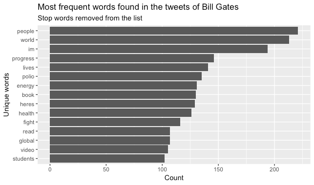
6. SHOW THE MOST FREQUENTLY USED HASHTAGS
You can do the same analysis with the hashtags. In this case, you'll want to use the hashtags variable from the rtweet package. A nice way to visualise these is using a word cloud as shown below.
          Gates_tweets_organic$hashtags <- as.character(Gates_tweets_organic$hashtags)
Gates_tweets_organic$hashtags <- gsub("c\\(", "", Gates_tweets_organic$hashtags)          set.seed(1234)
wordcloud(Gates_tweets_organic$hashtags, min.freq=5, scale=c(3.5, .5), random.order=FALSE, rot.per=0.35,
            colors=brewer.pal(8, "Dark2"))

7. SHOW THE ACCOUNTS FROM WHICH MOST RETWEETS ORIGINATE
Retweeting extensively from one account is usually not what someone looks for in a Twitter account. A helpful insight is therefore to monitor and understand from which accounts most retweets originate. The variable you'll want to analyse here is retweet_screen_name and the process to visualise it is similar to the one described previously using word clouds.
          set.seed(1234)
wordcloud(Gates_retweets$retweet_screen_name, min.freq=3, scale=c(2, .5), random.order=FALSE, rot.per=0.25,
colors=brewer.pal(8, "Dark2")) 
8. PERFORM A SENTIMENT ANALYSIS OF THE TWEETS
Finally, you may want to add a sentiment analysis at the end of your Twitter Analytics Report. This is easy to do with the package "syuzhet" and allows you to further deepen your analysis by grasping the tone of the tweets. No one likes a Twitter account that only spreads angry or sad tweets. Capturing the tone of your tweets and how they balance out is a good indication of your account's performance.
          library(syuzhet)          # Converting tweets to ASCII to trackle strange characters
tweets <- iconv(tweets, from="UTF-8", to="ASCII", sub="")          # removing retweets, in case needed
tweets <-gsub("(RT|via)((?:\\b\\w*@\\w+)+)","",tweets)          # removing mentions, in case needed
tweets <-gsub("@\\w+","",tweets)          ew_sentiment<-get_nrc_sentiment((tweets))
sentimentscores<-data.frame(colSums(ew_sentiment[,]))          names(sentimentscores) <- "Score"          sentimentscores <- cbind("sentiment"=rownames(sentimentscores),sentimentscores)          rownames(sentimentscores) <- NULL          ggplot(data=sentimentscores,aes(x=sentiment,y=Score))+
            geom_bar(aes(fill=sentiment),stat = "identity")+
            theme(legend.position="none")+
            xlab("Sentiments")+ylab("Scores")+
            ggtitle("Total sentiment based on scores")+
            theme_minimal()

Summary
In this article, I aimed to show how to extract and analyse tweets using the free-to-use programming software R. I hope you found this guide helpful to build your own Twitter Analytics Report that includes:
- Showing which tweets worked best and which didn't
- The ratio of organic tweets/replies/retweets, the time of tweet publication and the platforms from which tweets are published. These are all insights regarding the tweeting behaviour.
- The most frequent words used in the tweets, hashtags, from which accounts most retweets originate and a sentiment analysis capturing the tone of the tweets. These are all insights on the content of the tweets.
I regularly write articles about Data Science and Natural Language Processing. Follow me on Twitter or Medium to check out more articles like these or simply to keep updated about the next ones!
Posted by: clementinecalais.blogspot.com
Source: https://towardsdatascience.com/a-guide-to-mining-and-analysing-tweets-with-r-2f56818fdd16